import stockait as sai
import pandas as pd
본 글은 stockait 라이브러리를 사용하여 같은 방식으로 전처리한 데이터셋으로 각각 다른 머신러닝 모델을 학습하여 어떤 트레이더의 수익률이 가장 높게 나오는지 실험해보는 예제입니다.
1. 데이터 불러오기
⭐ 본 글에서 사용되는 주가 데이터셋 전처리는 생략하고, [stockait] stockait 사용하여 주가 예측 모델 학습하기 글과 같은 방식으로 전처리하여 저장한 데이터를 불러와서 사용하겠습니다.
df_time_series = pd.read_parquet("../../../../cha0716/time_series_0305.parquet")
df_time_series_scaled = pd.read_parquet("../../../../cha0716/time_series_scaled_0305.parquet")

df_time_series = df_time_series[~(df_time_series["Code"].isin(["33626K", "33637k", '33637K']))]
df_time_series_scaled = df_time_series_scaled[~(df_time_series_scaled["Code"].isin(["33626K", "33637k", '33637K']))]

df_time_series['Code'] = df_time_series['Code'].astype(str).str.zfill(6)
df_time_series_scaled['Code'] = df_time_series_scaled['Code'].astype(str).str.zfill(6)
불러온 데이터셋은 2016년 부터 2021년까지 div-close 방법으로 표준화된 시계열 데이터입니다.
data = df_time_series # Data Before Scaling
data_scaled = df_time_series_scaled # Data After Scaling

# train, test dataset split
train_data = data[(data['Date'] >= '2017-01-01') & (data['Date'] <= '2020-12-31')]
test_data = data[(data['Date'] >= '2021-01-01') & (data['Date'] <= '2021-12-31')]

# train, test dataset split (scaled)
train_data_scaled = data_scaled[(data_scaled['Date'] >= '2017-01-01') & (data_scaled['Date'] <= '2020-12-31')]
test_data_scaled = data_scaled[(data_scaled['Date'] >= '2021-01-01') & (data_scaled['Date'] <= '2021-12-31')]

print(train_data.shape, test_data.shape)
print(train_data_scaled.shape, test_data_scaled.shape)
(828290, 483) (217159, 483)
(828290, 483) (217159, 483)2017년 부터 2020년까지는 학습 데이터셋, 2021년은 시험 데이터셋으로 설정하였습니다.
2. Trader 정의
그 다음 트레이더를 정의합니다. 본 글에서는 글에서 정의했던 LightGBM, XGBoost, RandomForest, LSTM 모델을 그대로 사용하겠습니다.
lst_trader = [] 1) LightGBM
from lightgbm import LGBMClassifier

# conditional_buyer: Object that determines acquisition based on data filtering conditions
b1_lg = sai.ConditionalBuyer()

def sampling1(df): # Create a conditional function
    condition1 = (-0.3 <= df.D0_Change) & (df.D0_Change <= 0.3) # Remove exceptions that exceed upper and lower limits
    condition2 = (df.D0_Close * df.D0_Volume) >= 1000000000 # condition 1: Transaction amount of more than 1 billion won
    condition3 = (-0.05 >= df.D0_Change) | (0.05 <= df.D0_Change) # condition 2: Today's stock price change rate is more than 5%
    condition = condition1 & condition2 & condition3
    return condition

b1_lg.condition = sampling1  # Define the condition function directly (sampling1) and store it in the condition property


# machinelearning_buyer: Object that determines acquisition by machine learning model
b2_lg = sai.MachinelearningBuyer()

# Save user-defined models to algorithm properties
scale_pos_weight = round(72/28 , 2)
params = {  'random_state' : 42,
            'scale_pos_weight' : scale_pos_weight,
            'learning_rate' : 0.1,
            'num_iterations' : 1000,
            'max_depth' : 4,
            'n_jobs' : 30,
            'boost_from_average' : False,
            'objective' : 'binary' }

b2_lg.algorithm =  LGBMClassifier( **params )


# SubSeller: Object that determines selling all of the following days
sell_all = sai.SubSeller()


# Trader Object
t1 = sai.Trader()
t1.name = 'saiLightGBM' # Trader's name
t1.label = 'class&0.02' # Set the Trader dependent variable (do not set if it is regression analysis)
t1.buyer = sai.Buyer([b1_lg, b2_lg]) # [ conditional buyer, machinelearning buyer ]
t1.seller = sai.Seller(sell_all)

lst_trader.append(t1)
2) XGBoost
from xgboost import XGBClassifier

b1_xgb = sai.ConditionalBuyer()

def sampling2(df):
    condition1 = (-0.3 <= df.D0_Change) & (df.D0_Change <= 0.3)
    condition2 = (df.D0_Close * df.D0_Volume) >= 1000000000
    condition3 = (-0.05 >= df.D0_Change) | (0.05 <= df.D0_Change)
    condition = condition1 & condition2 & condition3
    return condition

b1_xgb.condition = sampling2


b2_xgb = sai.MachinelearningBuyer()

scale_pos_weight = round(72/28 , 2)
b2_xgb.algorithm = XGBClassifier(random_state = 42,
                   n_jobs=30,
                   scale_pos_weight=scale_pos_weight,
                   learning_rate=0.1,
                   max_depth=4,
                   n_estimators=1000,
                   )

sell_all = sai.SubSeller()


t2 = sai.Trader()
t2.name = 'saiXGboost'
t2.label = 'class&0.02'
t2.buyer = sai.Buyer([b1_xgb, b2_xgb])
t2.seller = sai.Seller(sell_all)

lst_trader.append(t2)
3) RandomForest
from sklearn.ensemble import RandomForestClassifier

b1_rf = sai.ConditionalBuyer()

def sampling3(df):
    condition1 = (-0.3 <= df.D0_Change) & (df.D0_Change <= 0.3)
    condition2 = (df.D0_Close * df.D0_Volume) >= 1000000000
    condition3 = (-0.05 >= df.D0_Change) | (0.05 <= df.D0_Change)
    condition = condition1 & condition2 & condition3
    return condition

b1_rf.condition = sampling3


b2_rf = sai.MachinelearningBuyer()

b2_rf.algorithm = RandomForestClassifier()


sell_all = sai.SubSeller()


t3 = sai.Trader()
t3.name = 'saiRandomForest'
t3.label = 'class&0.02'
t3.buyer = sai.Buyer([b1_rf, b2_rf])
t3.seller = sai.Seller(sell_all)

lst_trader.append(t3)
4) LSTM
from tensorflow import keras
import numpy as np

b1_ls = sai.ConditionalBuyer()

def sampling4(df):
    condition1 = (-0.3 <= df.D0_Change) & (df.D0_Change <= 0.3)
    condition2 = (df.D0_Close * df.D0_Volume) >= 1000000000
    condition3 = (-0.05 >= df.D0_Change) | (0.05 <= df.D0_Change)
    condition = condition1 & condition2 & condition3
    return condition

b1_ls.condition = sampling4


b2_ls = sai.MachinelearningBuyer()

# ⭐ User-defined functions (users who want deep learning modeling)
def transform(data): # A function that converts into a two-dimensional structure / data: list (lst_time_series)
    data_2d = []
    n_col = int(len(data[0]) / 10)
    for row in data:
        data_2d.append([])
        for i in range(0, len(row), n_col):
            data_2d[-1].append(row[i:i+n_col])

    return np.array(data_2d)


# Directly define a two-dimensional structure transformation function (transform) and store it in the data_transform property
b2_ls.data_transform = transform

model = keras.models.Sequential()
model.add(keras.layers.InputLayer(input_shape=(10, 48)))
model.add(keras.layers.LSTM(128, activation='selu', return_sequences=True))
model.add(keras.layers.Dropout(0.2))
model.add(keras.layers.LSTM(64, activation='selu', return_sequences=True))
model.add(keras.layers.Dropout(0.2))
model.add(keras.layers.LSTM(32, activation='selu', return_sequences=False))
model.add(keras.layers.Dropout(0.2))
model.add(keras.layers.Dense(1, activation='sigmoid'))

model.compile(optimizer=keras.optimizers.Adam(
    learning_rate=keras.optimizers.schedules.ExponentialDecay(0.05,decay_steps=100000,decay_rate=0.96)),
    loss="binary_crossentropy",
    metrics=['accuracy'])

b2_ls.algorithm =  model


sell_all = sai.SubSeller()


t4 = sai.Trader()
t4.name = 'saiLSTM'
t4.label = 'class&0.02'
t4.buyer = sai.Buyer([b1_ls, b2_ls])
t4.seller = sai.Seller(sell_all)

lst_trader.append(t4)
2023-04-02 10:53:25.764037: I tensorflow/core/platform/cpu_feature_guard.cc:193] This TensorFlow binary is optimized with oneAPI Deep Neural Network Library (oneDNN) to use the following CPU instructions in performance-critical operations: AVX2 FMA
To enable them in other operations, rebuild TensorFlow with the appropriate compiler flags.
2023-04-02 10:53:25.885853: E tensorflow/stream_executor/cuda/cuda_blas.cc:2981] Unable to register cuBLAS factory: Attempting to register factory for plugin cuBLAS when one has already been registered
2023-04-02 10:53:26.354422: W tensorflow/stream_executor/platform/default/dso_loader.cc:64] Could not load dynamic library 'libnvinfer.so.7'; dlerror: libnvinfer.so.7: cannot open shared object file: No such file or directory; LD_LIBRARY_PATH: /usr/local/cuda-11.6/lib64::/usr/local/cuda-11.5/lib64:/usr/local/cuda-11.5/targets/x86_64-linux/lib
2023-04-02 10:53:26.354479: W tensorflow/stream_executor/platform/default/dso_loader.cc:64] Could not load dynamic library 'libnvinfer_plugin.so.7'; dlerror: libnvinfer_plugin.so.7: cannot open shared object file: No such file or directory; LD_LIBRARY_PATH: /usr/local/cuda-11.6/lib64::/usr/local/cuda-11.5/lib64:/usr/local/cuda-11.5/targets/x86_64-linux/lib
2023-04-02 10:53:26.354484: W tensorflow/compiler/tf2tensorrt/utils/py_utils.cc:38] TF-TRT Warning: Cannot dlopen some TensorRT libraries. If you would like to use Nvidia GPU with TensorRT, please make sure the missing libraries mentioned above are installed properly.
2023-04-02 10:53:27.287623: E tensorflow/stream_executor/cuda/cuda_driver.cc:265] failed call to cuInit: CUDA_ERROR_NO_DEVICE: no CUDA-capable device is detected
2023-04-02 10:53:27.287685: I tensorflow/stream_executor/cuda/cuda_diagnostics.cc:156] kernel driver does not appear to be running on this host (ahnbi2): /proc/driver/nvidia/version does not exist
2023-04-02 10:53:27.288577: I tensorflow/core/platform/cpu_feature_guard.cc:193] This TensorFlow binary is optimized with oneAPI Deep Neural Network Library (oneDNN) to use the following CPU instructions in performance-critical operations: AVX2 FMA
To enable them in other operations, rebuild TensorFlow with the appropriate compiler flags.네개의 모델을 정의하였고 각각의 모델을 모두 lst_trader 안에 넣었습니다.
3. Trader(Model) 학슴 및 평가
1) 트레이더에 데이터셋 저장하기
트레이더 안에 데이터셋을 저장합니다.
sai.save_dataset(lst_trader, train_data, test_data, train_data_scaled, test_data_scaled)== saiLightGBM ==
== train_code_date: (828290, 2), test_code_date: (217159, 2) ==
== trainX: (828290, 480), testX: (217159, 480) ==
== trainX_scaled: (828290, 480), testX_scaled: (217159, 480) ==
== trainY: (828290,), testY: (217159,) ==
== trainY_classification: (828290,), testY_classification: (217159,) ==
== saiXGboost ==
== train_code_date: (828290, 2), test_code_date: (217159, 2) ==
== trainX: (828290, 480), testX: (217159, 480) ==
== trainX_scaled: (828290, 480), testX_scaled: (217159, 480) ==
== trainY: (828290,), testY: (217159,) ==
== trainY_classification: (828290,), testY_classification: (217159,) ==
== saiRandomForest ==
== train_code_date: (828290, 2), test_code_date: (217159, 2) ==
== trainX: (828290, 480), testX: (217159, 480) ==
== trainX_scaled: (828290, 480), testX_scaled: (217159, 480) ==
== trainY: (828290,), testY: (217159,) ==
== trainY_classification: (828290,), testY_classification: (217159,) ==
== saiLSTM ==
== train_code_date: (828290, 2), test_code_date: (217159, 2) ==
== trainX: (828290, 480), testX: (217159, 480) ==
== trainX_scaled: (828290, 480), testX_scaled: (217159, 480) ==
== trainY: (828290,), testY: (217159,) ==
== trainY_classification: (828290,), testY_classification: (217159,) ==
2) 모델 학습
각 트레이더에 정의되어있는 머신러닝 모델을 학습합니다.
sai.trader_train(lst_trader) == saiLightGBM Model Fitting Completed ==
== saiXGboost Model Fitting Completed ==
== saiRandomForest Model Fitting Completed ==
1268/1268 [==============================] - 18s 13ms/step - loss: 257227161600.0000 - accuracy: 0.6267
== saiLSTM Model Fitting Completed ==3) 모델 평가 및 임계값 설정
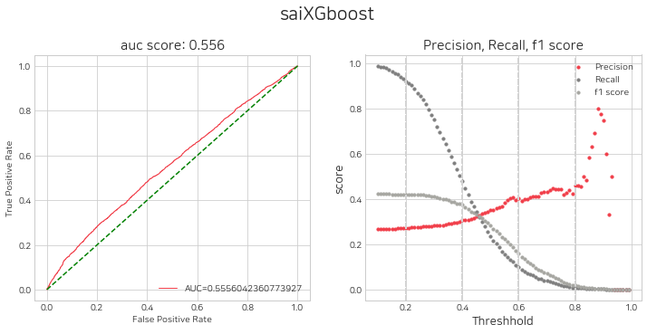
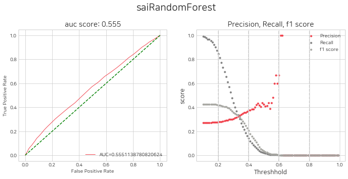
모델 평가
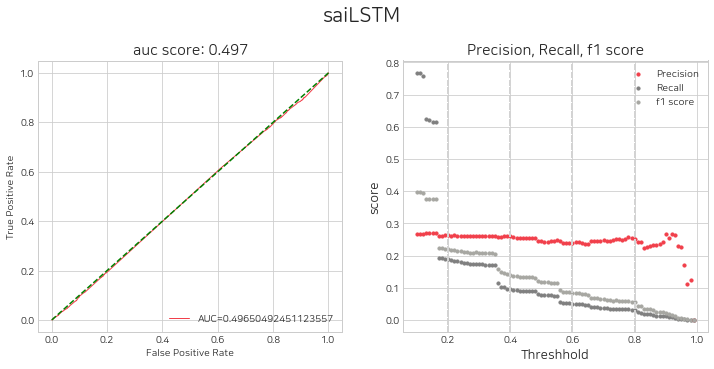
네개의 모델에 대하여 threshold 별 평가지표를 시각화 하고, 매수를 위한 임계값 설정을 고려합니다.
sai.get_eval_by_threshold(lst_trader)380/380 [==============================] - 2s 4ms/step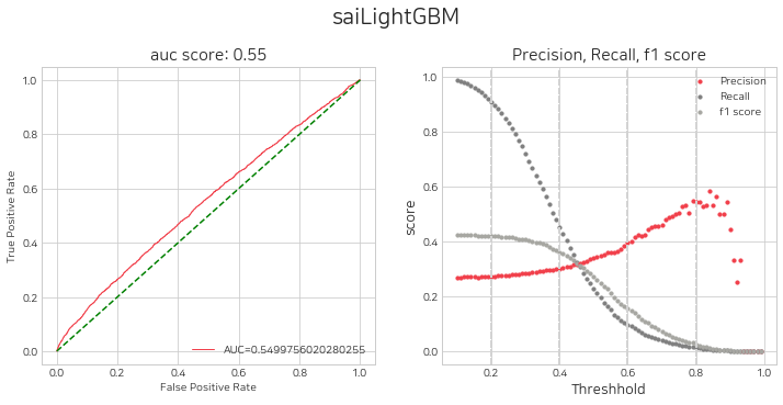
임계값 설정
위에서 판단한 threshold를 순서대로 lst_threshold에 넣어주고, histogram을 그려 수익성 검증을 할 수 있습니다. 예시로 0.8, 0.8, 0.6, 0.8 로 설정해주었고, 변경해가며 수익성 검증 실험을 지속적으로 해볼 수 있습니다.
sai.set_threshold(lst_trader, lst_threshold=[0.8, 0.8, 0.6, 0.8], histogram=True)Error: local variable 'threshold' referenced before assignment
380/380 [==============================] - 2s 4ms/step<Figure size 1152x720 with 0 Axes><Figure size 1152x720 with 0 Axes>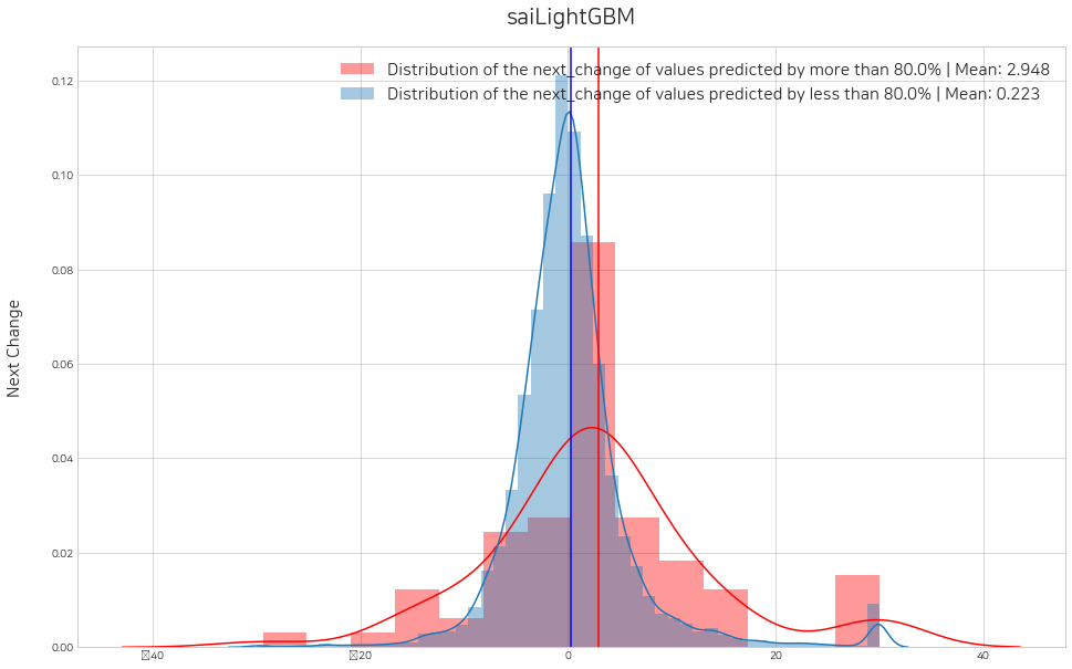
<Figure size 1152x720 with 0 Axes><Figure size 1152x720 with 0 Axes>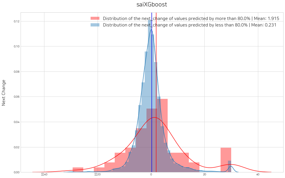
<Figure size 1152x720 with 0 Axes><Figure size 1152x720 with 0 Axes>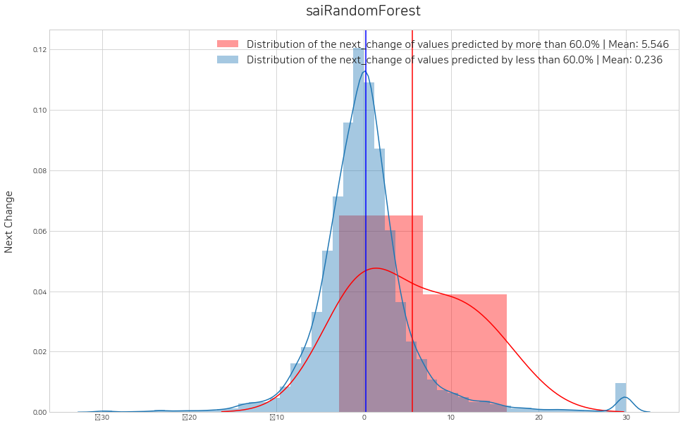
<Figure size 1152x720 with 0 Axes><Figure size 1152x720 with 0 Axes>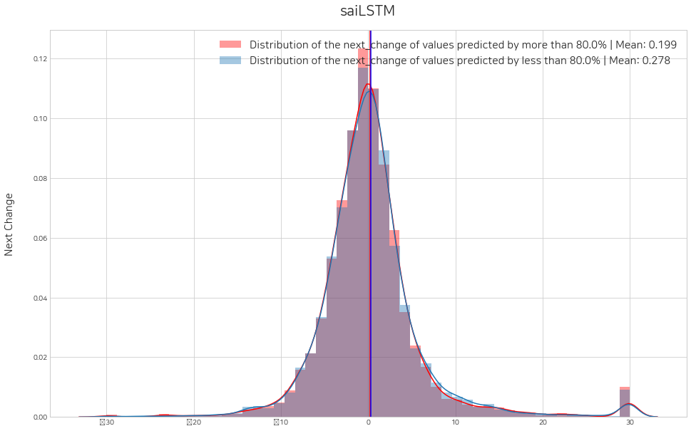
4. Back-Testing
1) 매매일지 작성
각각의 트레이더에서 모든 날짜에 대하여 매수 및 매도 기록을 생성합니다.
df_signal_all = sai.decision(lst_trader, dtype='test')
df_signal_all
217159it [00:06, 36183.33it/s]
217159it [00:05, 36418.57it/s]== saiLightGBM completed ==217159it [00:06, 35330.36it/s]
217159it [00:06, 35767.62it/s]== saiXGboost completed ==217159it [00:06, 35462.79it/s]
217159it [00:06, 35646.76it/s]== saiRandomForest completed ==
6787/6787 [==============================] - 30s 4ms/step217159it [00:05, 37334.97it/s]
217159it [00:05, 37169.70it/s]== saiLSTM completed ==| Trader_id | Date | Code | +(buy)/-(sell) | Amount | Close | |
|---|---|---|---|---|---|---|
| 0 | saiLightGBM | 2021-01-04 | 000020 | + | 0.0 | 19100.0 |
| 1 | saiLightGBM | 2021-01-05 | 000020 | + | 0.0 | 19400.0 |
| 2 | saiLightGBM | 2021-01-06 | 000020 | + | 0.0 | 19700.0 |
| 3 | saiLightGBM | 2021-01-07 | 000020 | + | 0.0 | 19700.0 |
| 4 | saiLightGBM | 2021-01-08 | 000020 | + | 0.0 | 19100.0 |
| ... | ... | ... | ... | ... | ... | ... |
| 217154 | saiLSTM | 2021-12-24 | 009900 | - | 1.0 | 30600.0 |
| 217155 | saiLSTM | 2021-12-27 | 009900 | - | 1.0 | 29900.0 |
| 217156 | saiLSTM | 2021-12-28 | 009900 | - | 1.0 | 29400.0 |
| 217157 | saiLSTM | 2021-12-29 | 009900 | - | 1.0 | 29850.0 |
| 217158 | saiLSTM | 2021-12-30 | 009900 | - | 1.0 | 30100.0 |
1737272 rows × 6 columns
2) 수익률 계산 시뮬레이션
위의 매매일지를 기반으로 각각의 트레이더의 모든 날짜에 대한 수익률을 계산합니다.
df_history_all = sai.simulation(df_signal_all, init_budget=10000000, init_stock={}, fee=0.01)
df_history_all
100%|███████████████████████████████████████████████████████████████████████████████████████████████▌| 247/248 [00:07<00:00, 33.88it/s]== saiLSTM completed ==100%|███████████████████████████████████████████████████████████████████████████████████████████████▌| 247/248 [00:07<00:00, 33.80it/s]== saiLightGBM completed ==100%|███████████████████████████████████████████████████████████████████████████████████████████████▌| 247/248 [00:07<00:00, 33.88it/s]== saiRandomForest completed ==100%|███████████████████████████████████████████████████████████████████████████████████████████████▌| 247/248 [00:07<00:00, 33.95it/s]== saiXGboost completed ==| Trader_id | Sell_date | Budget | Yield | Stock | |
|---|---|---|---|---|---|
| 0 | saiLSTM | 2021-01-04 | 10000000 | 0.000000 | {} |
| 1 | saiLSTM | 2021-01-05 | 10042066 | 0.420662 | {'000100': 3, '000660': 2, '001120': 10, '0013... |
| 2 | saiLSTM | 2021-01-06 | 9793093 | -2.069066 | {'000120': 1, '001250': 154, '001430': 27, '00... |
| 3 | saiLSTM | 2021-01-07 | 9830300 | -1.696992 | {'000220': 59, '001200': 107, '001250': 205, '... |
| 4 | saiLSTM | 2021-01-08 | 9808160 | -1.918394 | {'000540': 105, '001200': 67, '001380': 131, '... |
| ... | ... | ... | ... | ... | ... |
| 243 | saiXGboost | 2021-12-24 | 6110500 | -38.894995 | {'025620': 315} |
| 244 | saiXGboost | 2021-12-27 | 6110500 | -38.894995 | {} |
| 245 | saiXGboost | 2021-12-28 | 6110500 | -38.894995 | {} |
| 246 | saiXGboost | 2021-12-29 | 6110500 | -38.894995 | {} |
| 247 | saiXGboost | 2021-12-30 | 6110500 | -38.894995 | {} |
992 rows × 5 columns
3) Leader Board
트레이더의 최종 수익률 결과를 내림차순 정렬하여 데이터프레임으로 리더보드를 생성합니다.
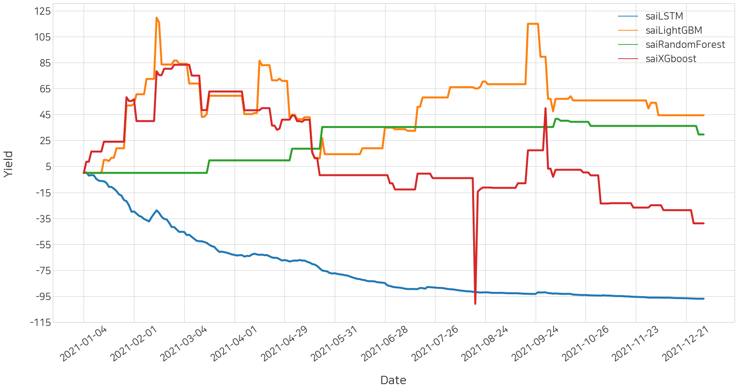
sai.leaderboard(df_history_all)| Trader_id | Yield | |
|---|---|---|
| 0 | saiLightGBM | 44.423725 |
| 1 | saiRandomForest | 29.597223 |
| 2 | saiXGboost | -38.894995 |
| 3 | saiLSTM | -96.950032 |
본 실험에서는 LightGBM의 수익률이 가장 높게 나왔으며, LSTM의 수익률이 가장 낮게 나왔습니다.
4) 수익률 결과 시각화
트레이더 별로 모든 날짜에 대한 수익률 추이를 확인할 수 있습니다.
sai.yield_plot(df_history_all)